Hierarchical Linear Model

2025-06-29

Introduction

This vignette estimates a hierarchical linear model with HART priors using bayesm.HART, applied to the orangeJuice scanner panel dataset from bayesm. The HART prior specifies the representative store as a sum-of-trees function of observed demographics, Delta(Z_i), whereas the conventional specification uses the linear form Delta^\\top Z_i.

Orange Juice Scanner Panel Data

The orangeJuice dataset contains weekly store-level scanner data for 83 stores. We observe log-sales, prices of 11 brands, and deal/feature indicators. Store demographics (income, education, ethnicity, household size, etc.) serve as covariates $Z_i$. Following Montgomery (1997), we estimate a log-log demand model for brand 1 (Tropicana Premium 64 oz), so coefficients are directly interpretable as price elasticities.

# Load dependencies
library(bayesm.HART)
library(bayesm)
# Data wrangling and plotting utilities
library(tidyr)
library(dplyr)
library(ggplot2)

# Load orange juice scanner panel data
data(orangeJuice)
yx <- orangeJuice[["yx"]]
storedemo <- orangeJuice[["storedemo"]]

# Subset to brand 1 (Tropicana)
brand1 <- yx[yx[["brand"]] == 1, ]

# Build per-store regdata (following bayesm::orangeJuice documentation)
store_ids <- storedemo[["STORE"]]
nreg <- length(store_ids)
regdata <- vector("list", length = nreg)
price_cols <- paste0("price", 1:11)
for (i in 1:nreg) {
  si <- brand1[brand1[["store"]] == store_ids[i], ]
  y <- si[["logmove"]]
  X <- cbind(1, log(as.matrix(si[, price_cols])), si[["deal"]], si[["feat"]])
  colnames(X) <- c("Intercept", paste0("Log Price ", 1:11), "Deal", "Feature")
  regdata[[i]] <- list(y = y, X = X)
}

# Store-level demographics as Z (omit STORE id column, de-mean)
Z <- as.matrix(storedemo[, -1])
Z <- t(t(Z) - colMeans(Z)) # de-mean covariates as required by bayesm

# Final data object
Data <- list(regdata = regdata, Z = Z)

MCMC Estimation

We fit both the HART model (Wiemann, 2025) and a conventional linear hierarchical model (Rossi et al., 2009). Both estimate store-specific coefficients $\beta_i$ via a hierarchical linear model; they differ only in their specification of $\Delta(\cdot)$. A short chain of 5000 iterations is used here for illustration; longer chains should be run in practice.

# MCMC parameters
R <- 5000
burn <- 250
keep <- 1
Mcmc <- list(R = R, keep = keep)

model_cache_file <- file.path(
  vignette_cache_dir,
  sprintf("oj-linear-R%s-keep%s.rds", R, keep)
)

model_cache_ok <- FALSE
if (file.exists(model_cache_file)) {
  model_cache <- tryCatch(readRDS(model_cache_file), error = function(e) NULL)
  model_cache_ok <- !is.null(model_cache) &&
    !is.null(model_cache$out_hart) && !is.null(model_cache$out_lin)
  if (model_cache_ok) {
    out_hart <- model_cache$out_hart
    out_lin  <- model_cache$out_lin
    cat("Loaded cached model draws from:", model_cache_file, "\n")
  }
}

if (!model_cache_ok) {
  out_hart <- bayesm.HART::rhierLinearMixture(
    Data = Data, Mcmc = Mcmc,
    Prior = list(
      ncomp = 1,
      bart = list(num_trees = 20) # new HART prior parameters
    )
  )

  out_lin <- bayesm.HART::rhierLinearMixture(
    Data = Data, Mcmc = Mcmc,
    Prior = list(ncomp = 1)
  )

  saveRDS(
    list(out_hart = out_hart, out_lin = out_lin, generated_at = Sys.time()),
    model_cache_file
  )
  cat("Saved model draws cache to:", model_cache_file, "\n")
}

We use the log-likelihood trace as a basic MCMC diagnostic.

burnin_draws <- ceiling(burn / keep) 

mcmc_data <- data.frame(
  Iteration = (1:length(out_hart$loglike)) * keep,
  HART = out_hart$loglike,
  Linear = out_lin$loglike
) %>% 
  pivot_longer(cols = c("HART", "Linear"), names_to = "Model", values_to = "LogLikelihood")

ggplot(mcmc_data, aes(x = Iteration, y = LogLikelihood, color = Model)) +
  geom_line(alpha = 0.8) +
  geom_vline(xintercept = burn, linetype = "dashed", color = "black") +
  scale_color_manual(values = c("HART" = "blue", "Linear" = "red")) +
  theme_classic(base_size = 16) +
  labs(title = "Log-Likelihood Trace Plots", x = "MCMC Iteration", y = "Log-Likelihood") +
  theme(legend.title = element_blank(), 
        legend.position = "bottom",
        legend.text = element_text(size = 16))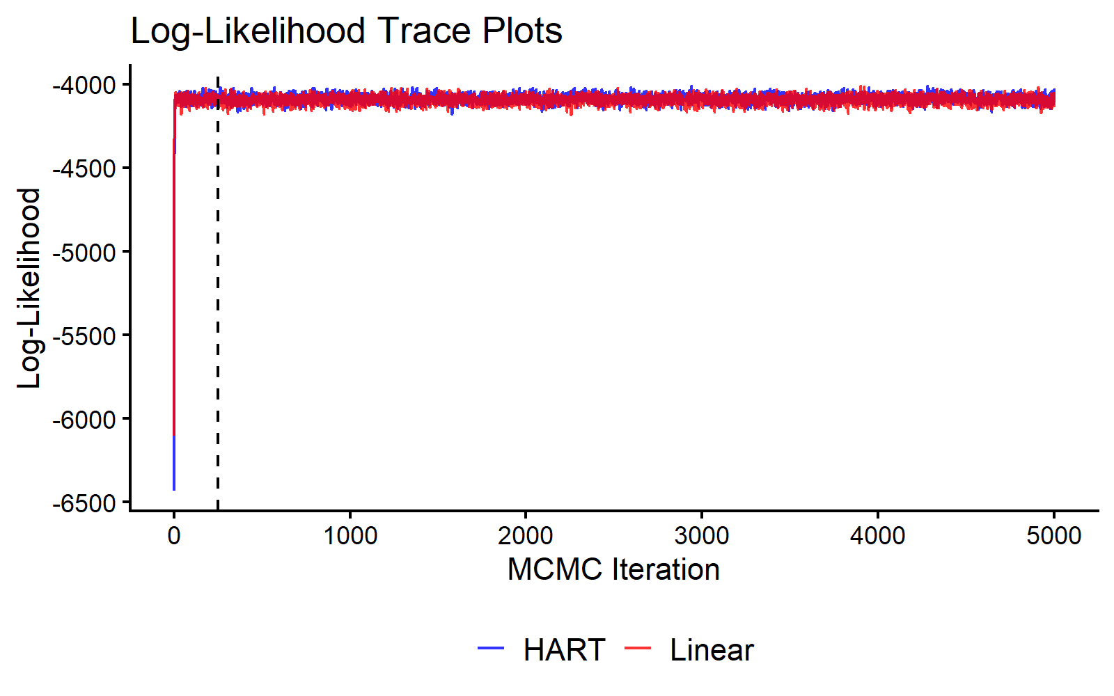

MCMC Traceplot of the Log Likelihood.

Posterior Inference about Store-level Coefficients

We compare posterior distributions of the own-price elasticity for two stores: Store 25 (high-income, highly educated area) and Store 79 (lower-income, high ethnic diversity).

selected_stores <- c(25, 79)
coef_indx <- 2 # "Log Price 1" = own-price elasticity
coef_name <- "Own-Price Elasticity"

# Create a combined factor for filling histograms
beta_draws <- bind_rows(
  as.data.frame(t(out_hart$betadraw[selected_stores, coef_indx, -c(1:burnin_draws)])) %>% 
    mutate(Model = "HART", Draw = row_number()),
  as.data.frame(t(out_lin$betadraw[selected_stores, coef_indx, -c(1:burnin_draws)])) %>% 
    mutate(Model = "Linear", Draw = row_number())
)
colnames(beta_draws)[1:2] <- paste("Store", selected_stores)

beta_draws_long <- beta_draws %>%
  pivot_longer(
    cols = starts_with("Store"), 
    names_to = "Store", 
    values_to = "Coefficient"
  ) %>% 
  mutate(
      Model = factor(Model, levels = c("Linear", "HART")), # Control facet order
      Group = interaction(Store, Model)
  )

# Define colors
model_fills <- c(
    "Store 25.Linear" = "lightcoral", "Store 79.Linear" = "darkred",
    "Store 25.HART" = "lightblue", "Store 79.HART" = "darkblue"
)
model_colors <- c(
    "Store 25.Linear" = "red", "Store 79.Linear" = "darkred",
    "Store 25.HART" = "blue", "Store 79.HART" = "darkblue"
)

# Calculate means
means <- beta_draws_long %>%
  group_by(Group, Model) %>%
  summarise(mean_val = mean(Coefficient), .groups = "drop")

ggplot(beta_draws_long, aes(x = Coefficient, fill = Group)) +
  geom_histogram(aes(y = after_stat(density)), alpha = 0.6, bins = 45, 
                 position = "identity", color = "black", linewidth = 0.3) +
  geom_vline(data = means, aes(xintercept = mean_val, color = Group),
             linetype = "dashed", linewidth = 1.2) +
  facet_wrap(~Model) +
  scale_fill_manual(name = "Store", values = model_fills,
                    breaks = c("Store 25.Linear", "Store 79.Linear", 
                               "Store 25.HART", "Store 79.HART"),
                    labels = c("Store 25", "Store 79", 
                               "Store 25", "Store 79")) +
  scale_color_manual(values = model_colors, guide = "none") +
  theme_classic(base_size = 16) +
  theme(axis.title = element_text(size = 18), legend.position = "top",
        legend.title = element_blank(),
        strip.text = element_text(size = 16, face = "bold"),
        strip.background = element_rect(fill = "grey90", color = "black")) +
    labs(title = paste("Selected Posterior Distributions of Store-level", coef_name),
    x = "Elasticity", y = "Density")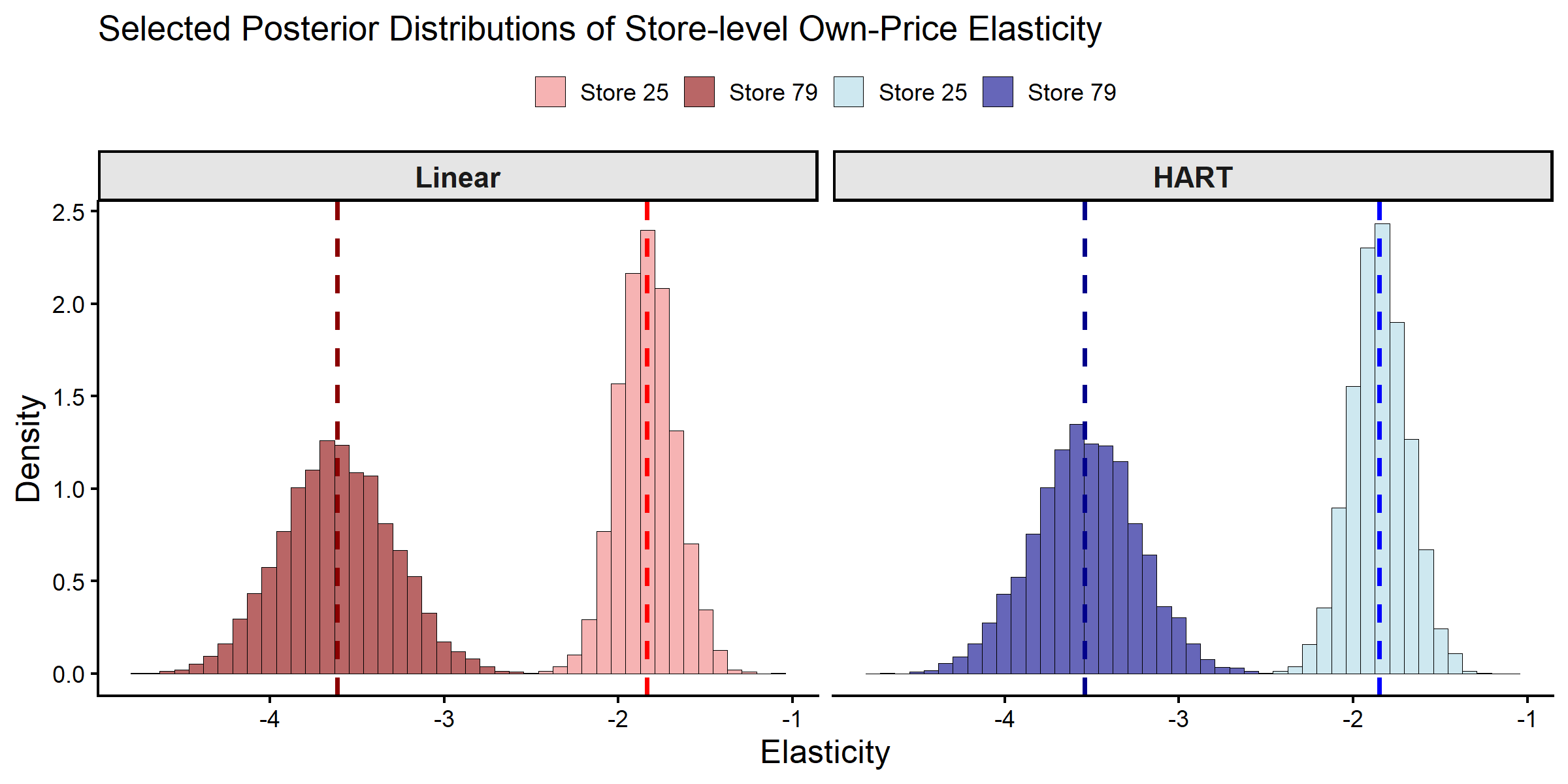

Posterior Distributions of Store-level Own-Price Elasticities.

# Extract posterior draws for the selected stores and coefficient
hart_draws_25 <- out_hart$betadraw[25, coef_indx, -c(1:burnin_draws)]
hart_draws_79 <- out_hart$betadraw[79, coef_indx, -c(1:burnin_draws)]
lin_draws_25 <- out_lin$betadraw[25, coef_indx, -c(1:burnin_draws)]
lin_draws_79 <- out_lin$betadraw[79, coef_indx, -c(1:burnin_draws)]

# Create summary table
summary_results <- data.frame(
  Model = c("Linear", "Linear", "HART", "HART"),
  Store = c("25", "79", "25", "79"),
  Mean = c(mean(lin_draws_25), mean(lin_draws_79), 
           mean(hart_draws_25), mean(hart_draws_79)),
  SD = c(sd(lin_draws_25), sd(lin_draws_79), 
         sd(hart_draws_25), sd(hart_draws_79))
)

print(summary_results, digits = 3)
#>    Model Store  Mean    SD
#> 1 Linear    25 -1.84 0.167
#> 2 Linear    79 -3.61 0.320
#> 3   HART    25 -1.85 0.166
#> 4   HART    79 -3.54 0.304

Both models produce similar individual-level elasticity estimates for the selected stores. With about 117 weekly observations per store, the individual likelihood contributes most of the posterior information at the store level in this application.

Posterior Inference on Store Segment Coefficients

The models differ in how they characterize the expected coefficient $\Delta(Z)$ for a representative store with demographics $Z$. We compare these segment-level predictions for the same two stores, using the predict function.

# We predict for all stores
DeltaZ_hat_hart <- predict(out_hart, newdata = list(Z = Z), type = "DeltaZ+mu", burn = burnin_draws)
DeltaZ_hat_lin <- predict(out_lin, newdata = list(Z = Z), type = "DeltaZ+mu", burn = burnin_draws)

deltaZ_draws <- bind_rows(
  as.data.frame(t(DeltaZ_hat_hart[selected_stores, coef_indx, ])) %>% 
    mutate(Model = "HART", Draw = row_number()),
  as.data.frame(t(DeltaZ_hat_lin[selected_stores, coef_indx, ])) %>% 
    mutate(Model = "Linear", Draw = row_number())
)
colnames(deltaZ_draws)[1:2] <- c("Segment 1", "Segment 2")

deltaZ_draws_long <- deltaZ_draws %>%
  pivot_longer(
    cols = starts_with("Segment"), 
    names_to = "Store_Segment", 
    values_to = "Coefficient"
  ) %>% 
  mutate(
      Model = factor(Model, levels = c("Linear", "HART")), # Control facet order
      Group = interaction(Store_Segment, Model)
  )
  
# Update color definitions to match segment terminology
model_fills <- c(
    "Segment 1.Linear" = "lightcoral", "Segment 2.Linear" = "darkred",
    "Segment 1.HART" = "lightblue", "Segment 2.HART" = "darkblue"
)
model_colors <- c(
    "Segment 1.Linear" = "red", "Segment 2.Linear" = "darkred",
    "Segment 1.HART" = "blue", "Segment 2.HART" = "darkblue"
)

# Calculate means
means_deltaZ <- deltaZ_draws_long %>%
  group_by(Group, Model) %>%
  summarise(mean_val = mean(Coefficient), .groups = "drop")

ggplot(deltaZ_draws_long, aes(x = Coefficient, fill = Group)) +
  geom_histogram(aes(y = after_stat(density)), alpha = 0.6, bins = 45, 
                 position = "identity", color = "black", linewidth = 0.3) +
  geom_vline(data = means_deltaZ, aes(xintercept = mean_val, color = Group),
             linetype = "dashed", linewidth = 1.2) +
  facet_wrap(~Model) +
  scale_fill_manual(name = "Store Segment", values = model_fills,
                    breaks = c("Segment 1.Linear", "Segment 2.Linear", 
                               "Segment 1.HART", "Segment 2.HART"),
                    labels = c("Segment 1", "Segment 2", 
                               "Segment 1", "Segment 2")) +
  scale_color_manual(values = model_colors, guide = "none") +
  theme_classic(base_size = 16) +
  theme(axis.title = element_text(size = 18), legend.position = "top",
        legend.title = element_blank(),
        strip.text = element_text(size = 16, face = "bold"),
        strip.background = element_rect(fill = "grey90", color = "black")) +
         labs(title = "Posterior Distributions of Expected Own-Price Elasticities",
     x = "Elasticity", y = "Density")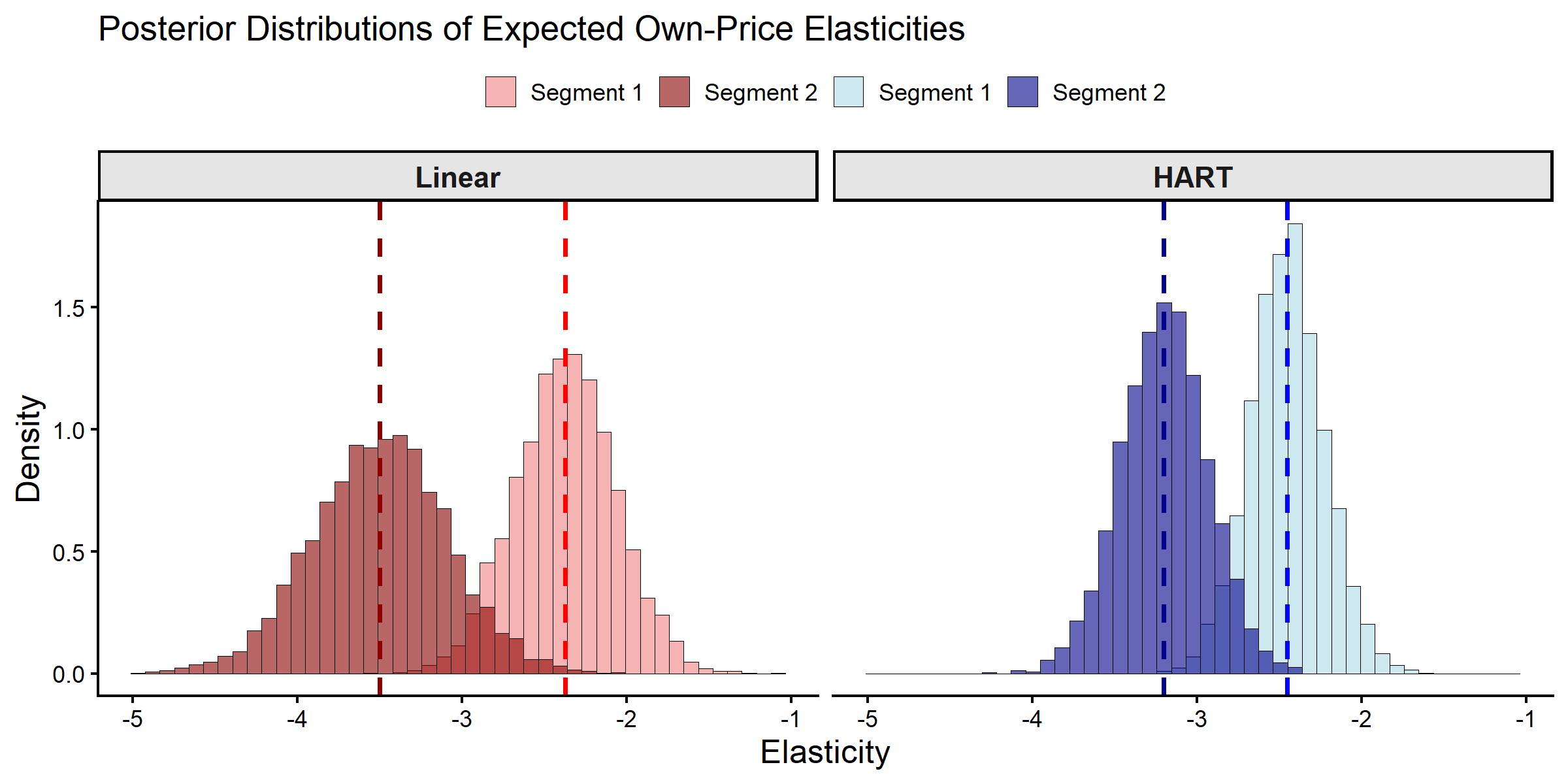

Posterior Distributions of Expected Store Segment Coefficients.

# Extract expected coefficients for the two segments
deltaZ_summary <- data.frame(
  Segment = c("Segment 1 (High Income, High Education)", 
              "Segment 2 (Low Income, High Ethnic Diversity)"),
  Linear_Mean = c(mean(DeltaZ_hat_lin[25, coef_indx, ]), 
                  mean(DeltaZ_hat_lin[79, coef_indx, ])),
  Linear_SD = c(sd(DeltaZ_hat_lin[25, coef_indx, ]), 
                sd(DeltaZ_hat_lin[79, coef_indx, ])),
  HART_Mean = c(mean(DeltaZ_hat_hart[25, coef_indx, ]), 
                mean(DeltaZ_hat_hart[79, coef_indx, ])),
  HART_SD = c(sd(DeltaZ_hat_hart[25, coef_indx, ]), 
              sd(DeltaZ_hat_hart[79, coef_indx, ]))
)

print(deltaZ_summary, digits = 3)
#>                                         Segment Linear_Mean Linear_SD HART_Mean
#> 1       Segment 1 (High Income, High Education)       -2.37     0.305     -2.45
#> 2 Segment 2 (Low Income, High Ethnic Diversity)       -3.50     0.412     -3.20
#>   HART_SD
#> 1   0.227
#> 2   0.263

# Calculate differences between segments
cat("\nDifferences between segments:\n")
#> 
#> Differences between segments:
cat("Linear approach difference:", 
    deltaZ_summary$Linear_Mean[2] - deltaZ_summary$Linear_Mean[1], "\n")
#> Linear approach difference: -1.127546
cat("HART approach difference:", 
    deltaZ_summary$HART_Mean[2] - deltaZ_summary$HART_Mean[1], "\n")
#> HART approach difference: -0.750117

The linear specification restricts segment means to an affine function of demographics. HART allows nonlinear and interaction structure in Z through Delta(Z).

References

Montgomery, Alan L. (1997). “Creating Micro-Marketing Pricing Strategies Using Supermarket Scanner Data.” Marketing Science 16(4), pp. 315–337.

Rossi, Peter E., Greg M. Allenby, and Robert McCulloch (2009). Bayesian Statistics and Marketing. Reprint. Wiley Series in Probability and Statistics. Chichester: Wiley.

Wiemann, Thomas (2025). “Personalization with HART.” Working paper.