Get Started

2025-06-29

Introduction

This vignette illustrates how to estimate a hierarchical logit model with HART priors using the bayesm.HART package. Following Application I in Wiemann (2025), the HART logit model is applied to the bank conjoint dataset of Allenby and Ginter (1995) on out-of-state credit card design.

bayesm.HART uses a Hierarchical Additive Regression Tree (HART) prior. This specifies the representative consumer as a nonparametric function of observed characteristics. This vignette contrasts that HART logit specification with a conventional hierarchical logit model where the representative consumer is linear in characteristics.

The rest of the vignette proceeds as follows: 1. Load and prepare data for use with bayesm and bayesm.HART 2. Run MCMC chains for fully Bayesian inference 3. Posterior inference on respondent-level part-worths 4. Posterior inference on consumer segment part-worths

Conjoint Data of Allenby and Ginter (1995)

We use the bank dataset in bayesm, originally analyzed by Allenby and Ginter (1995). The data include responses from 946 customers in a telephone conjoint on credit card attributes. Respondents were part of a new-market (“out-of-state”) targeting exercise and each provided 13 to 17 binary choice responses. The dataset contains 14,799 binary responses plus respondent age, income, and gender.

The code below prepares the data for bayesm and bayesm.HART. Both packages use the same data structure.

# Load dependencies
library(bayesm.HART)
library(bayesm)
#> 
#> Attaching package: 'bayesm'
#> The following objects are masked from 'package:bayesm.HART':
#> 
#>     rhierLinearMixture, rhierMnlRwMixture, rhierNegbinRw
# Data wrangling and plotting utilities
library(tidyr)
library(dplyr)
#> 
#> Attaching package: 'dplyr'
#> The following objects are masked from 'package:stats':
#> 
#>     filter, lag
#> The following objects are masked from 'package:base':
#> 
#>     intersect, setdiff, setequal, union
library(ggplot2)

# Load and prepare data from the 'bank' dataset (same as bayesm)
data(bank)
choiceAtt <- bank$choiceAtt
hh <- levels(factor(choiceAtt$id))
nhh <- length(hh)
lgtdata <- vector("list", length = nhh)
for (i in 1:nhh) {
    y = 2 - choiceAtt[choiceAtt[,1]==hh[i], 2]
    nobs = length(y)
    X_temp = as.matrix(choiceAtt[choiceAtt[,1]==hh[i], c(3:16)])
    X = matrix(0, nrow = nrow(X_temp) * 2, ncol = ncol(X_temp))
    X[seq(1, nrow(X), by = 2), ] = X_temp
    lgtdata[[i]] = list(y=y, X=X)
}
Z <- as.matrix(bank$demo[, -1]) # omit id
Z <- t(t(Z) - colMeans(Z)) # de-mean covariates as required by bayesm

# Final data object (same as bayesm)
Data <- list(lgtdata = lgtdata, Z = Z, p = 2)

MCMC Estimation

We apply two models to the conjoint data: the HART logit model (Wiemann, 2025) and a conventional linear hierarchical logit model (Rossi et al., 2009). Both models are motivated by a latent utility model of consumer choice. The models differ only in how they capture preference heterogeneity: the linear approach models the relationship between a respondent’s characteristics and their part-worths as a linear function $\Delta^\top Z_i$, while HART uses a flexible sum-of-trees factor model $\Delta(Z_i)$ to capture rich nonlinearities and interactions.

The code below sets MCMC hyperparameters and runs both samplers. For vignette runtime, we use 5,000 iterations (longer chains are recommended in practice). Both models are estimated with rhierMnlRwMixture; the HART specification adds the bart entry in Prior. We use 20 trees per factor and keep other hyperparameters at defaults.

Because this walkthrough focuses on in-sample predictions at observed respondent covariates Z, we set store_trees = FALSE for HART to skip tree serialization during fitting and use the cached unique-Z prediction path. If you need out-of-sample predictions on unseen Z* or mode = "prior" with type = "choice_probs", fit with store_trees = TRUE.

# Specify MCMC parameters
R <- 5000
burn <- 250
keep <- 1
Mcmc <- list(R = R, keep = keep)

model_cache_file <- file.path(
  vignette_cache_dir,
  sprintf("bank-get-started-R%s-keep%s.rds", R, keep)
)

model_cache_ok <- FALSE
if (file.exists(model_cache_file)) {
  model_cache <- tryCatch(readRDS(model_cache_file), error = function(e) NULL)
  model_cache_ok <- !is.null(model_cache) &&
    !is.null(model_cache$out_hart) && !is.null(model_cache$out_lin)
  if (model_cache_ok) {
    out_hart <- model_cache$out_hart
    out_lin  <- model_cache$out_lin
    cat("Loaded cached model draws from:", model_cache_file, "\n")
  }
}
#> Loaded cached model draws from: C:\Users\twiem\AppData\Local/R/cache/R/bayesm.HART/vignettes/bank-get-started-R5000-keep1.rds

if (!model_cache_ok) {
  # Fit HART Logit (cache-first prediction mode; no tree serialization)
  out_hart <- bayesm.HART::rhierMnlRwMixture(
    Data,
    Prior = list(ncomp = 1, bart = list(num_trees = 20), store_trees = FALSE),
    Mcmc
  )

  # Fit conventional Linear Hierarchical Logit
  out_lin <- bayesm::rhierMnlRwMixture(Data, Prior = list(ncomp = 1), Mcmc)

  saveRDS(
    list(out_hart = out_hart, out_lin = out_lin, generated_at = Sys.time()),
    model_cache_file
  )
  cat("Saved model draws cache to:", model_cache_file, "\n")
}

A simple diagnostic is the log-likelihood trace over MCMC iterations. In this run, both chains appear to mix after the burn-in cutoff in the traceplot below.

burnin_draws <- ceiling(burn / keep) 

mcmc_data <- data.frame(
  Iteration = (1:length(out_hart$loglike)) * keep,
  HART = out_hart$loglike,
  Linear = out_lin$loglike
) %>% 
  pivot_longer(cols = c("HART", "Linear"), names_to = "Model", values_to = "LogLikelihood")

ggplot(mcmc_data, aes(x = Iteration, y = LogLikelihood, color = Model)) +
  geom_line(alpha = 0.8) +
  geom_vline(xintercept = burn, linetype = "dashed", color = "black") +
  scale_color_manual(values = c("HART" = "blue", "Linear" = "red")) +
  theme_classic(base_size = 16) +
  labs(title = "Log-Likelihood Trace Plots", x = "MCMC Iteration", y = "Log-Likelihood") +
  theme(legend.title = element_blank(), 
        legend.position = "bottom",
        legend.text = element_text(size = 16))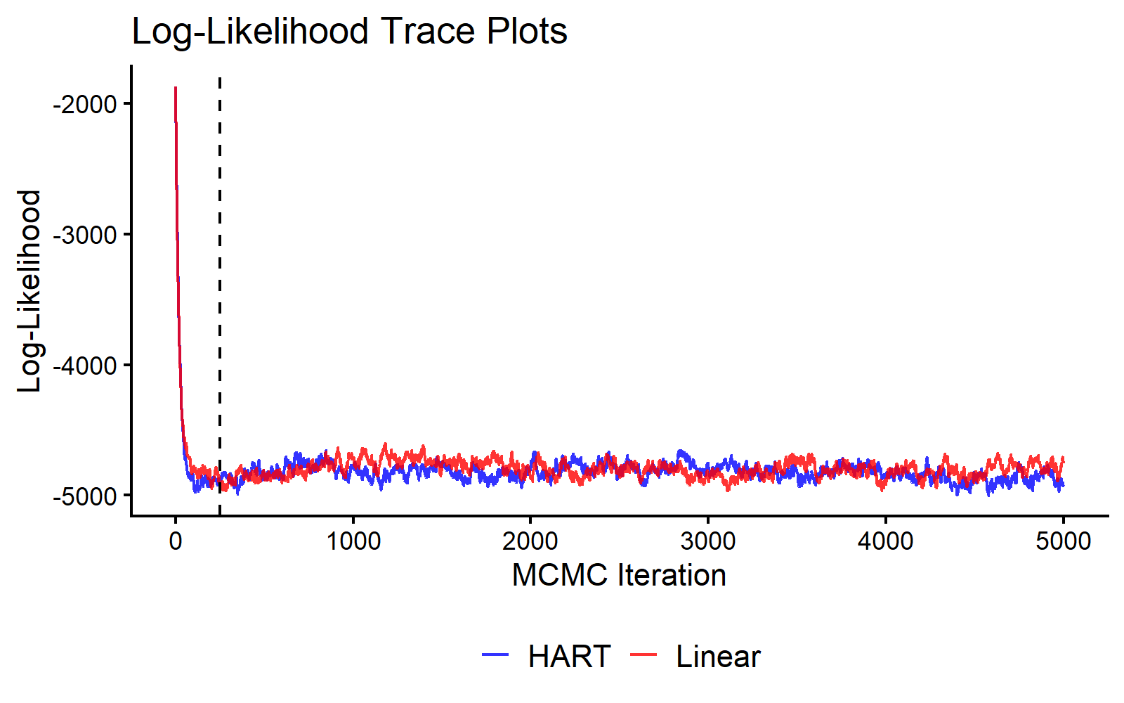

MCMC Traceplot of the Log Likelihood.

Posterior Inference on Respondent-level Part-Worths

With the MCMC draws complete, we characterize the posterior estimates for individual-level coefficients (part-worths). To illustrate the models, we examine the posterior distributions for two specific respondents: Respondent 146 (an older woman with low income) and Respondent 580 (a middle-aged man with moderate income). The comparison focuses on the out-of-state bank attribute, which represents a key design challenge for the bank’s expansion strategy.

selected_resp <- c(146, 580)
coef_indx <- 10 # "Interest" coefficient
coef_name <- colnames(bank$choiceAtt[, 3:16])[coef_indx]

# Create a combined factor for filling histograms
beta_draws <- bind_rows(
  as.data.frame(t(out_hart$betadraw[selected_resp, coef_indx, -c(1:burnin_draws)])) %>% 
    mutate(Model = "HART", Draw = row_number()),
  as.data.frame(t(out_lin$betadraw[selected_resp, coef_indx, -c(1:burnin_draws)])) %>% 
    mutate(Model = "Linear", Draw = row_number())
)
colnames(beta_draws)[1:2] <- paste("Respondent", selected_resp)

beta_draws_long <- beta_draws %>%
  pivot_longer(
    cols = starts_with("Respondent"), 
    names_to = "Respondent", 
    values_to = "Coefficient"
  ) %>% 
  mutate(
      Model = factor(Model, levels = c("Linear", "HART")), # Control facet order
      Group = interaction(Respondent, Model)
  )

# Define colors
model_fills <- c(
    "Respondent 146.Linear" = "lightcoral", "Respondent 580.Linear" = "darkred",
    "Respondent 146.HART" = "lightblue", "Respondent 580.HART" = "darkblue"
)
model_colors <- c(
    "Respondent 146.Linear" = "red", "Respondent 580.Linear" = "darkred",
    "Respondent 146.HART" = "blue", "Respondent 580.HART" = "darkblue"
)

# Calculate means
means <- beta_draws_long %>%
  group_by(Group, Model) %>%
  summarise(mean_val = mean(Coefficient), .groups = "drop")

ggplot(beta_draws_long, aes(x = Coefficient, fill = Group)) +
  geom_histogram(aes(y = after_stat(density)), alpha = 0.6, bins = 45, 
                 position = "identity", color = "black", linewidth = 0.3) +
  geom_vline(data = means, aes(xintercept = mean_val, color = Group),
             linetype = "dashed", linewidth = 1.2) +
  facet_wrap(~Model) +
  scale_fill_manual(name = "Respondent", values = model_fills,
                    breaks = c("Respondent 146.Linear", "Respondent 580.Linear", 
                               "Respondent 146.HART", "Respondent 580.HART"),
                    labels = c("Respondent 146", "Respondent 580", 
                               "Respondent 146", "Respondent 580")) +
  scale_color_manual(values = model_colors, guide = "none") +
  theme_classic(base_size = 16) +
  theme(axis.title = element_text(size = 18), legend.position = "top",
        legend.title = element_blank(),
        strip.text = element_text(size = 16, face = "bold"),
        strip.background = element_rect(fill = "grey90", color = "black")) +
    labs(title = paste("Selected Posterior Distributions of Individual Out-of-State Part-Worths"),
    x = "Coefficient Value", y = "Density")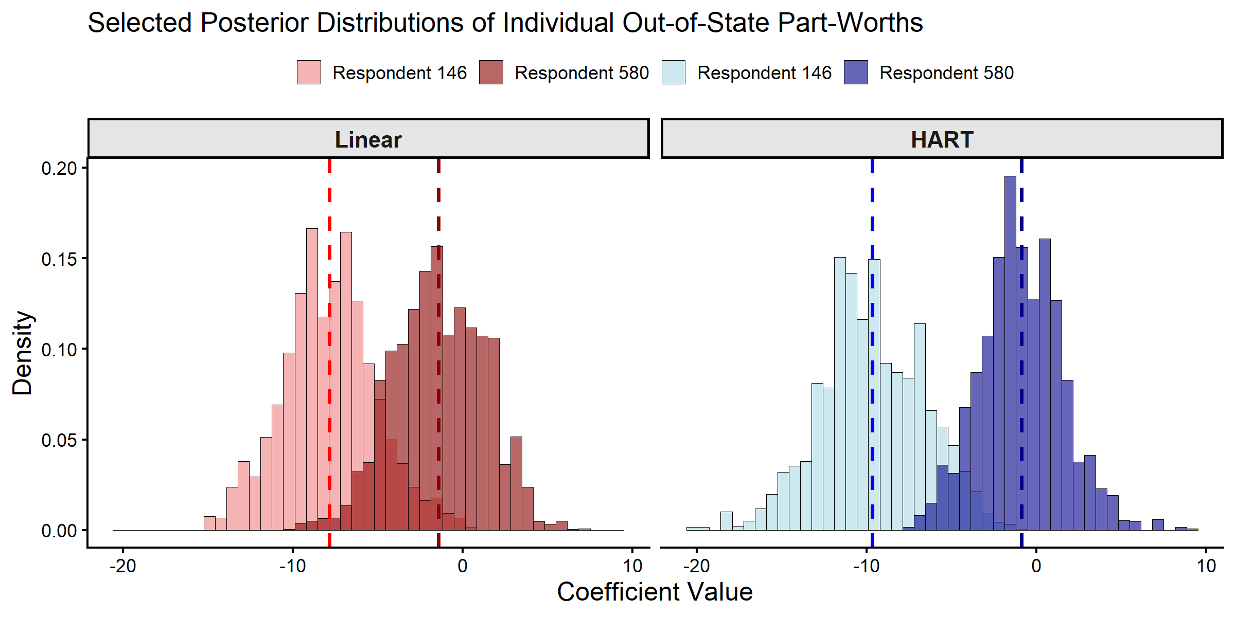

Posterior Distributions of Individual-level Part-Worths.

# Extract posterior draws for the selected respondents and coefficient
hart_draws_146 <- out_hart$betadraw[146, coef_indx, -c(1:burnin_draws)]
hart_draws_580 <- out_hart$betadraw[580, coef_indx, -c(1:burnin_draws)]
lin_draws_146 <- out_lin$betadraw[146, coef_indx, -c(1:burnin_draws)]
lin_draws_580 <- out_lin$betadraw[580, coef_indx, -c(1:burnin_draws)]

# Create summary table
summary_results <- data.frame(
  Model = c("Linear", "Linear", "HART", "HART"),
  Respondent = c("146", "580", "146", "580"),
  Mean = c(mean(lin_draws_146), mean(lin_draws_580), 
           mean(hart_draws_146), mean(hart_draws_580)),
  SD = c(sd(lin_draws_146), sd(lin_draws_580), 
         sd(hart_draws_146), sd(hart_draws_580))
)

print(summary_results, digits = 3)
#>    Model Respondent  Mean   SD
#> 1 Linear        146 -7.84 2.74
#> 2 Linear        580 -1.41 2.69
#> 3   HART        146 -9.67 3.05
#> 4   HART        580 -0.87 2.43

Both models produce similar individual-level part-worth estimates for these two respondents. This similarity is expected: when respondents have many choice profiles (here, between 13 and 17), their individual-level posterior estimates are primarily driven by their own choice data rather than the first-stage prior.

Differences between HART and linear hierarchical models are typically more visible when individual-level data are limited and estimation depends more on the representative consumer. The next section compares representative-consumer posteriors for the selected segments.

Posterior Inference on Consumer Segment Part-Worths

The model estimates how part-worths vary with demographics $Z$, where $\Delta(Z)$ represents the expected part-worth for a “representative” respondent with characteristics $Z$.

To illustrate the differences between the models, we predict preferences for two granularly-defined consumer segments. Segment 1 is defined as older female respondents with low income, while Segment 2 is defined as middle-aged male respondents with moderate income. We use the predict function to get the posterior draws of the expected part-worths for these selected segments.

# We predict for all respondents (seen Z rows -> cached fast path)
DeltaZ_hat_hart <- predict(out_hart, newdata = list(Z = Z), type = "DeltaZ+mu", burn = burnin_draws)
class(out_lin) <- "rhierMnlRwMixture" # allows bayesm model to use bayesm.HART methods 
DeltaZ_hat_lin <- predict(out_lin, newdata = list(Z = Z), type = "DeltaZ+mu", burn = burnin_draws)

deltaZ_draws <- bind_rows(
  as.data.frame(t(DeltaZ_hat_hart[selected_resp, coef_indx, ])) %>% 
    mutate(Model = "HART", Draw = row_number()),
  as.data.frame(t(DeltaZ_hat_lin[selected_resp, coef_indx, ])) %>% 
    mutate(Model = "Linear", Draw = row_number())
)
colnames(deltaZ_draws)[1:2] <- c("Segment 1", "Segment 2")

deltaZ_draws_long <- deltaZ_draws %>%
  pivot_longer(
    cols = starts_with("Segment"), 
    names_to = "Consumer_Segment", 
    values_to = "Coefficient"
  ) %>% 
  mutate(
      Model = factor(Model, levels = c("Linear", "HART")), # Control facet order
      Group = interaction(Consumer_Segment, Model)
  )
  
# Update color definitions to match segment terminology
model_fills <- c(
    "Segment 1.Linear" = "lightcoral", "Segment 2.Linear" = "darkred",
    "Segment 1.HART" = "lightblue", "Segment 2.HART" = "darkblue"
)
model_colors <- c(
    "Segment 1.Linear" = "red", "Segment 2.Linear" = "darkred",
    "Segment 1.HART" = "blue", "Segment 2.HART" = "darkblue"
)

# Calculate means
means_deltaZ <- deltaZ_draws_long %>%
  group_by(Group, Model) %>%
  summarise(mean_val = mean(Coefficient), .groups = "drop")

ggplot(deltaZ_draws_long, aes(x = Coefficient, fill = Group)) +
  geom_histogram(aes(y = after_stat(density)), alpha = 0.6, bins = 45, 
                 position = "identity", color = "black", linewidth = 0.3) +
  geom_vline(data = means_deltaZ, aes(xintercept = mean_val, color = Group),
             linetype = "dashed", linewidth = 1.2) +
  facet_wrap(~Model) +
  scale_fill_manual(name = "Consumer Segment", values = model_fills,
                    breaks = c("Segment 1.Linear", "Segment 2.Linear", 
                               "Segment 1.HART", "Segment 2.HART"),
                    labels = c("Segment 1", "Segment 2", 
                               "Segment 1", "Segment 2")) +
  scale_color_manual(values = model_colors, guide = "none") +
  theme_classic(base_size = 16) +
  theme(axis.title = element_text(size = 18), legend.position = "top",
        legend.title = element_blank(),
        strip.text = element_text(size = 16, face = "bold"),
        strip.background = element_rect(fill = "grey90", color = "black")) +
         labs(title = "Posterior Distributions of Expected Out-of-State Part-Worths",
     x = "Coefficient Value", y = "Density")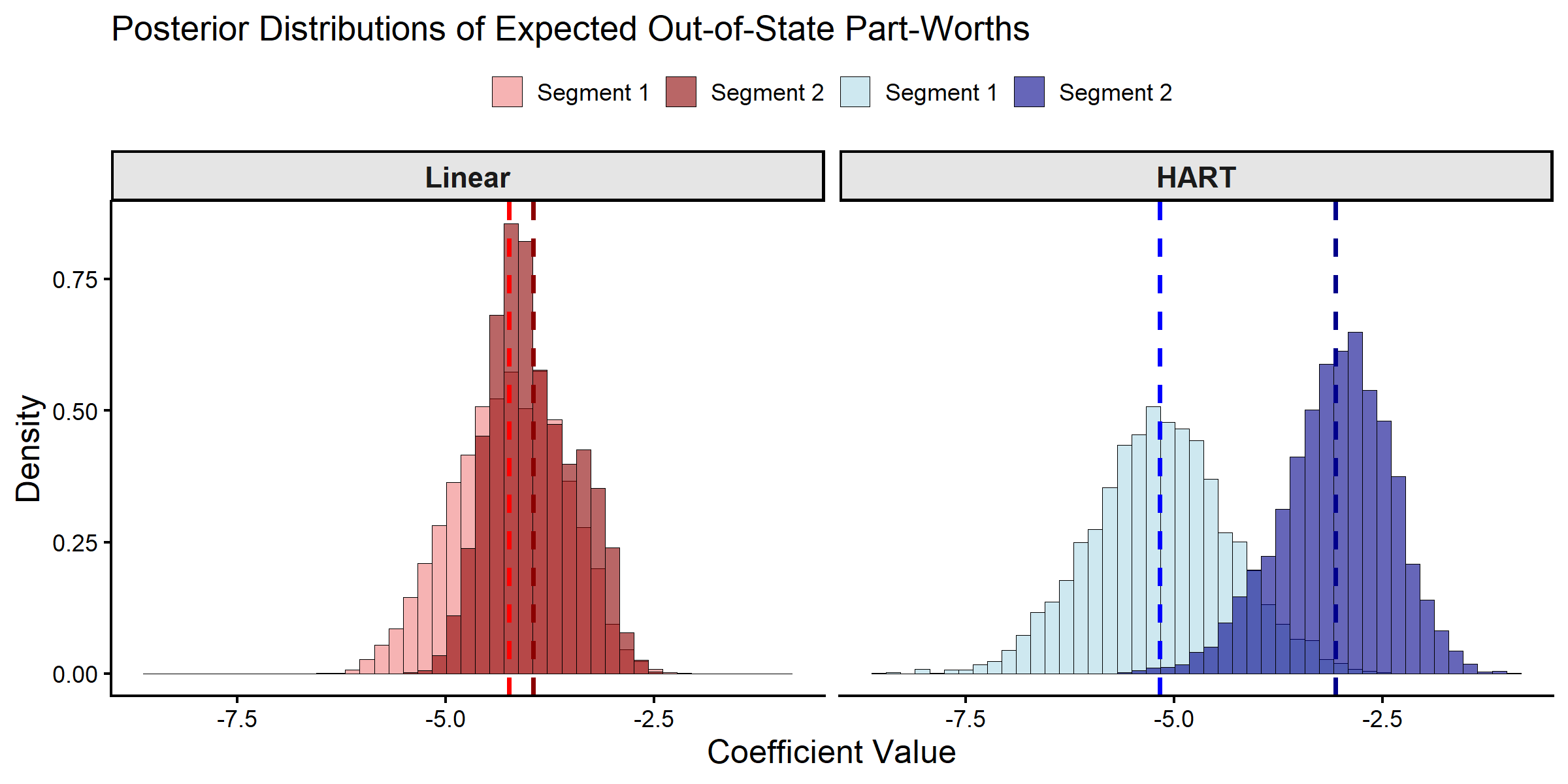

Posterior Distributions of Expected Part-Worths.

# Extract expected part-worths for the two segments
deltaZ_summary <- data.frame(
  Segment = c("Segment 1 (Older Women, Low Income)", 
              "Segment 2 (Middle-aged Men, Moderate Income)"),
  Linear_Mean = c(mean(DeltaZ_hat_lin[146, coef_indx, ]), 
                  mean(DeltaZ_hat_lin[580, coef_indx, ])),
  Linear_SD = c(sd(DeltaZ_hat_lin[146, coef_indx, ]), 
                sd(DeltaZ_hat_lin[580, coef_indx, ])),
  HART_Mean = c(mean(DeltaZ_hat_hart[146, coef_indx, ]), 
                mean(DeltaZ_hat_hart[580, coef_indx, ])),
  HART_SD = c(sd(DeltaZ_hat_hart[146, coef_indx, ]), 
              sd(DeltaZ_hat_hart[580, coef_indx, ]))
)

print(deltaZ_summary, digits = 3)
#>                                        Segment Linear_Mean Linear_SD HART_Mean
#> 1          Segment 1 (Older Women, Low Income)       -4.24     0.665     -5.17
#> 2 Segment 2 (Middle-aged Men, Moderate Income)       -3.95     0.508     -3.06
#>   HART_SD
#> 1   0.836
#> 2   0.663

# Calculate differences between segments
cat("\nDifferences between segments:\n")
#> 
#> Differences between segments:
cat("Linear approach difference:", 
    deltaZ_summary$Linear_Mean[2] - deltaZ_summary$Linear_Mean[1], "\n")
#> Linear approach difference: 0.2937976
cat("HART approach difference:", 
    deltaZ_summary$HART_Mean[2] - deltaZ_summary$HART_Mean[1], "\n")
#> HART approach difference: 2.109128

# Additional variance diagnostics for the selected out-of-state coefficient.
post_ids <- (burnin_draws + 1):dim(out_hart$betadraw)[3]

# 1) Respondent-level posterior variance of beta_i.
resp_var <- data.frame(
  Model = c("Linear", "Linear", "HART", "HART"),
  Target = c("Respondent 146 beta", "Respondent 580 beta",
             "Respondent 146 beta", "Respondent 580 beta"),
  Variance = c(
    var(out_lin$betadraw[146, coef_indx, post_ids]),
    var(out_lin$betadraw[580, coef_indx, post_ids]),
    var(out_hart$betadraw[146, coef_indx, post_ids]),
    var(out_hart$betadraw[580, coef_indx, post_ids])
  )
)

# 2) Segment-level posterior variance of Delta(Z)+mu.
seg_var <- data.frame(
  Model = c("Linear", "Linear", "HART", "HART"),
  Target = c("Segment 1 Delta+mu", "Segment 2 Delta+mu",
             "Segment 1 Delta+mu", "Segment 2 Delta+mu"),
  Variance = c(
    var(DeltaZ_hat_lin[146, coef_indx, ]),
    var(DeltaZ_hat_lin[580, coef_indx, ]),
    var(DeltaZ_hat_hart[146, coef_indx, ]),
    var(DeltaZ_hat_hart[580, coef_indx, ])
  )
)

# 3) Posterior variance of the implied random-effects covariance entry Sigma[k,k].
sigma_entry_draws_hart <- sapply(out_hart$nmix$compdraw[post_ids], function(draw) {
  rooti <- draw[[1]]$rooti
  solve(crossprod(rooti))[coef_indx, coef_indx]
})
sigma_entry_draws_lin <- sapply(out_lin$nmix$compdraw[post_ids], function(draw) {
  rooti <- draw[[1]]$rooti
  solve(crossprod(rooti))[coef_indx, coef_indx]
})

sigma_var <- data.frame(
  Model = c("Linear", "HART"),
  Mean = c(mean(sigma_entry_draws_lin), mean(sigma_entry_draws_hart)),
  Variance = c(var(sigma_entry_draws_lin), var(sigma_entry_draws_hart)),
  SD = c(sd(sigma_entry_draws_lin), sd(sigma_entry_draws_hart)),
  Q05 = c(quantile(sigma_entry_draws_lin, 0.05), quantile(sigma_entry_draws_hart, 0.05)),
  Q95 = c(quantile(sigma_entry_draws_lin, 0.95), quantile(sigma_entry_draws_hart, 0.95))
)

print(resp_var, digits = 3)
#>    Model              Target Variance
#> 1 Linear Respondent 146 beta     7.52
#> 2 Linear Respondent 580 beta     7.26
#> 3   HART Respondent 146 beta     9.32
#> 4   HART Respondent 580 beta     5.90
print(seg_var, digits = 3)
#>    Model             Target Variance
#> 1 Linear Segment 1 Delta+mu    0.442
#> 2 Linear Segment 2 Delta+mu    0.258
#> 3   HART Segment 1 Delta+mu    0.700
#> 4   HART Segment 2 Delta+mu    0.440
print(sigma_var, digits = 3)
#>    Model Mean Variance    SD  Q05  Q95
#> 1 Linear 3.96    0.704 0.839 2.70 5.32
#> 2   HART 4.18    0.883 0.939 2.87 6.06

if (!is.null(out_hart$acceptrbeta)) {
  cat("\nHART MH acceptrbeta (%):", round(out_hart$acceptrbeta, 2), "\n")
}
#> 
#> HART MH acceptrbeta (%): 23.03

For the selected segments and focal coefficient, the posterior distributions differ across model specifications. In this vignette run, the HART posterior means for segment-level expected part-worths are more separated than the corresponding linear-model means. This pattern is consistent with the broader function class in HART, where Delta(Z_i) allows nonlinear and interaction structure in demographics.

Quantifying Explained Variance ($R^2$)

To quantify explained demographic heterogeneity, we compute a Bayesian R^2 measure. This is the fraction of latent preference heterogeneity explained by observed demographics Z.

Because this is a hierarchical model, the “total” variance of the part-worths is mathematically decomposed into the variance of the predictions $\Delta(Z_i)$ across the population (the explained variance) and the unobserved structural heterogeneity $\Sigma_{kk}$ (the residual variance). By evaluating this at every MCMC iteration, we obtain a full posterior distribution for the $R^2$.

smry_hart <- summary(out_hart, Z = Z, burn = burnin_draws, coefs = coef_indx)
smry_lin  <- summary(out_lin, Z = Z, burn = burnin_draws, coefs = coef_indx)

r2_data <- bind_rows(
  data.frame(Model = "HART", R2 = smry_hart$r2$R2_draws[, 1]),
  data.frame(Model = "Linear", R2 = smry_lin$r2$R2_draws[, 1])
) %>%
  mutate(Model = factor(Model, levels = c("Linear", "HART")))

ggplot(r2_data, aes(x = R2, fill = Model)) +
  geom_density(alpha = 0.6, color = "black") +
  scale_fill_manual(values = c("Linear" = "red", "HART" = "blue")) +
  scale_x_continuous(labels = scales::percent_format(accuracy = 1)) +
  theme_classic(base_size = 16) +
  labs(title = "Variance Explained by Demographics",
       x = expression(R^2), y = "Density") +
  theme(legend.title = element_blank(), legend.position = "top")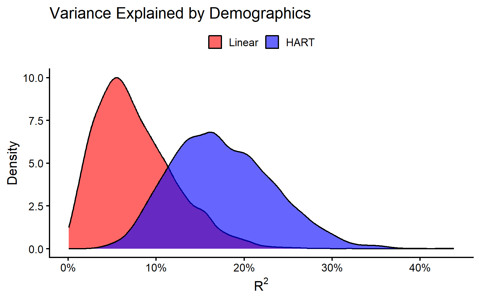

Posterior Distributions of Explained Variance ($R^2$) for Out-of-State Preferences.

cat("Posterior Mean R² (Linear):", round(smry_lin$r2$R2_mean * 100, 2), "%\n")
#> Posterior Mean R² (Linear): 7.62 %
cat("Posterior Mean R² (HART)  :", round(smry_hart$r2$R2_mean * 100, 2), "%\n")
#> Posterior Mean R² (HART)  : 17.56 %

The density plot summarizes posterior draws of explained variance for the focal coefficient under each specification. In this run, posterior R^2 draws are shifted upward under HART relative to the linear specification, indicating higher explained heterogeneity for the same demographic inputs.

References

Allenby, Greg M. and James L. Ginter (1995). “Using Extremes to Design Products and Segment Markets.” Journal of Marketing Research 32.4, pp. 392–403.

Rossi, Peter E., Greg M. Allenby, and Robert McCulloch (2009). Bayesian Statistics and Marketing. Reprint. Wiley Series in Probability and Statistics. Chichester: Wiley.

Wiemann, Thomas (2025). “Personalization with HART.” Working paper.