Plot Summarized Marginal Effects

Creates a ggplot visualization of the summarized marginal effects from one or more summary.marginal_effects objects.

Usage

# S3 method for class 'summary.marginal_effects'
plot(
  x,
  ...,
  coef_index = 1,
  ci_level = 0.95,
  plot_axis_var = NULL,
  xlab = NULL,
  ylab = NULL,
  title = NULL,
  color_values = NULL,
  linetype_values = NULL,
  fill_values = NULL,
  show_legend = TRUE,
  x_name = NULL
)

Arguments

x

An object of class "summary.marginal_effects".

...

Additional named objects of class "summary.marginal_effects" to be plotted alongside x. The names will be used in the legend.

coef_index

Integer, the index of the coefficient (beta) to plot. Defaults to 1.

ci_level

Numeric (0 < ci_level < 1), the credible interval level to display as a ribbon (e.g., 0.95 for a 95% CI). Requires the corresponding quantiles (e.g., q2.5 and q97.5 or q25 and q975) to be present in the summary_df of the input object(s). Defaults to 0.95.

plot_axis_var

Character, the name of the column in summary_df to use on the x-axis (must be one of the z_val_* columns derived from the non-NA columns of the original z_values input to marginal_effects). If NULL (default), the function will use the first column found in x$summary_df that matches the pattern ^z_val_[0-9]+$.

xlab

Character, custom label for the x-axis. If NULL (default), the label will be the value of plot_axis_var.

ylab

Character, custom label for the y-axis. Defaults to describing the mean effect of the selected coefficient.

title

Character, custom plot title. If NULL (default), the title will indicate the coefficient and the variable plotted on the x-axis.

color_values

Named character vector for custom colors (e.g., c("Model A" = "blue", "Model B" = "red")). If NULL, default ggplot colors are used.

linetype_values

Named character vector for custom linetypes (e.g., c("Model A" = "solid", "Model B" = "dashed")). If NULL, default ggplot linetypes are used.

fill_values

Named character vector for custom ribbon fills (e.g., c("Model A" = "blue", "Model B" = "red")). If NULL, default ggplot fills derived from colors are used.

show_legend

Logical, should the legend be displayed? Defaults to TRUE.

x_name

Character, optional name to assign to the primary object x in the legend. If NULL (default), the function attempts to infer the name.

Value

A ggplot object.

Details

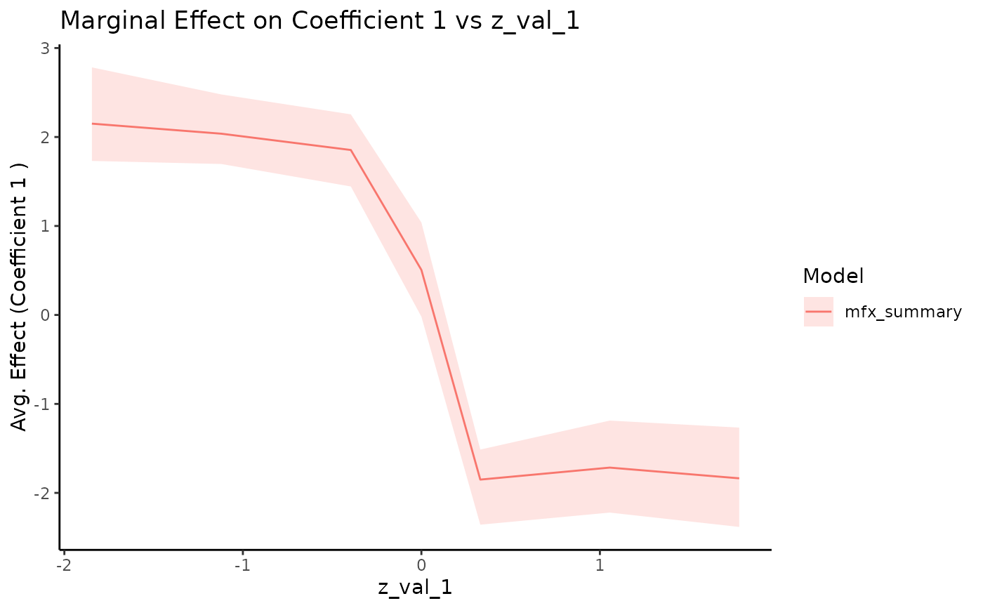
This function plots the specified coefficient's posterior mean and credible interval against the variable specified by plot_axis_var.

If the original marginal_effects call used a z_values matrix that varied across multiple dimensions (resulting in multiple z_val_* columns in the summary_df), this plot will show the relationship against the chosen plot_axis_var, overlaying the results from all combinations of the other varying dimensions. For instance, if z_val_1 and z_val_2 exist and plot_axis_var = "z_val_1", the plot will show lines for each distinct value of z_val_2 (implicitly, as they will be overlaid).

To visualize the effect along one dimension conditional on specific values of other dimensions, you should filter the summary_df within the summary.marginal_effects object before passing it to this function.

Examples

# --- Full Example Sequence for Plotting ---
# Requires ggplot2 and bayesm.HART
if (requireNamespace("bayesm.HART", quietly = TRUE) && 
    requireNamespace("ggplot2", quietly = TRUE)) {

  # 1. Simulate Data (using a step function for beta_i)
  # Define simulation parameters
  nlgt_sim <- 200; nT_sim <- 20; p_sim <- 3; nz_sim <- 2
  nXa_sim <- 1; nXd_sim <- 0; const_sim <- TRUE
  # Calculate expected ncoef based on parameters
  ncoef_sim <- const_sim*(p_sim - 1) + (p_sim - 1)*nXd_sim + nXa_sim
  # Define arguments for the step function (using defaults from sim_hier_mnl)
  step_args_ex <- list(
    cutoff = 0,               # Default cutoff
    beta_1 = rep(-2, ncoef_sim), # Value above cutoff (default in sim_hier_mnl)
    beta_2 = rep(2, ncoef_sim),  # Value below cutoff (default in sim_hier_mnl)
    Z_index = 1               # Step based on Z1
  )
  sim_data <- bayesm.HART::sim_hier_mnl(nlgt = nlgt_sim, nT = nT_sim, p = p_sim, nz = nz_sim,
                                    nXa = nXa_sim, nXd = nXd_sim, const = const_sim,
                                    seed = 123,
                                    beta_func_type = "step",
                                    beta_func_args = step_args_ex # Pass the full list
                                    )
  Data <- list(p = sim_data$p, lgtdata = sim_data$lgtdata, Z = sim_data$Z)
  # Use actual ncoef from simulation output for consistency
  ncoef <- sim_data$true_values$dimensions$ncoef 

  # 2. Fit Model (minimal run for example)
  Prior <- list(ncomp = 1,
                bart = list(num_trees = 10,
                            num_cut = 10))
  Mcmc <- list(R = 500, keep = 1, nprint = 0)
  fit <- try(bayesm.HART::rhierMnlRwMixture(Data = Data, Prior = Prior, 
                                        Mcmc = Mcmc, 
                                        r_verbose = FALSE), silent = TRUE)

  if (!inherits(fit, "try-error")) {
    # 3. Define Grid (Vary Z1, which drives the step function)
    target_z_index <- 1
    grid_z1 <- sort(c(seq(min(Data$Z[, target_z_index]), 
                           max(Data$Z[, target_z_index]), 
                           length.out = 6), 0)) # Use more points for step
    z_grid <- matrix(NA, nrow = length(grid_z1), ncol = ncol(Data$Z))
    z_grid[, target_z_index] <- grid_z1

    # 4. Calculate Marginal Effects
    mfx_result <- marginal_effects(fit, 
                                     z_values = z_grid, 
                                     Z =Data$Z, 
                                     burn = 200, 
                                     verbose = FALSE)

    # 5. Summarize Marginal Effects
    mfx_summary <- summary(mfx_result, probs = c(0.025, 0.5, 0.975))

    # 6. Plot the Summary (showing effect of Z1 on coef 1)
    # Ensure the axis variable name matches the column in summary_df
    plot_var_name <- paste0("z_val_", target_z_index) 
    try(plot(mfx_summary, coef_index = 1, plot_axis_var = plot_var_name), silent = TRUE)

  } else {
    message("Model fitting failed in example, skipping plotting.")
  }
} else {
  message("Requires bayesm.HART and ggplot2 packages for examples.")
}